LQR Control of a Self Balancing Robot

In this post we're improving our self-balancing robot project, by introducing a Linear-Quadratic Regulator (LQR) to significantly improve stability and handling. We'll go through the entire derivation and implementation process, leveraging the Python terminal within Pictorus which makes all of this really easy.

Motivation

Previously, we introduced the design of a self-balancing robot that we stabilized with PID control. This is a very common first pass, since it's simple to implement and intuitive to tune.

However, there's plenty of reasons why PID often doesn't cut it. While fun to fiddle with, it can be difficult to reason through the behavior and limits of a PID controller. It can also be difficult to manage multiple control objectives, and the usual approach (nested or parallel PID loops) tend to fight each, rather than work together. Enter the Linear Quadratic Regulator.

Linear Quadratic Regulation

Linear Quadratic Regulators (LQR) are a class of optimal controllers that are really good at balancing multiple control objectives for linear dynamic systems. Meaning, if we can model our robot as a system of linear equations, LQR is the defacto process to drive that system toward some desired state.

Quick side note for control nerds - LQR is essentially the inverse of a Kalman Filter. A Kalman Filter is also known as a Linear Quadratic Estimator, using that same system of equations (with the help of some mathematical magic) to predict future states given noisy measurements. LQR closes the loop on such a system, and the LQR/Kalman pair are called the LQG Problem. They are often used together for computationally efficient, optimal control, dating back to the Apollo program.

Because LQR mathematically maps how each state affects every other, it's more systematic than PID at balancing multiple control goals. In our case, it "understands" how a change in pitch angle also affects velocity, so it strives for pitch angles which simultaneously nudge both pitch and velocity toward our desired goal, rather than letting those two objectives fight one another.

Furthermore, LQR lets us weigh different objectives relative to each other, so we can prioritize pitch angle (necessary to stay upright) over desired velocity. And since it understands how all of these control goals affect the magnitude of our control output, LQR also comes built in with a simple way to penalize control "effort". This means with a single variable we can make the entire control response more snappy or less snappy, which can have a big impact on power consumption and actuator lifetime.

Lastly, the math underpinning LQR allows us to derive statements about the factors of safety implied by our control solution. Both gain margin (safety against un-modeled system dynamics) and phase margin (safety against un-modeled lag in the system) are helpful metrics when engineers need to defend their control design. LQR's popularity is due in large part to how all these various features are relatively straightforward to compute from a given set of state equations.

However, everything discussed so far assumes a linear system, but in reality very few applications are truly linear. Non-linearities (in our case, trigonometric sine functions) essentially null and void the LQR warranty, so control design often entails linearization about some desired state (in our case, a vertical pendulum). Linearized controllers only guarantee performance near that linearization point, so large deviations can cause the control response to diverge.

Finally, all of these theoretical guarantees are only as good as their underlying dynamics model. If the equations of motion don't adequately capture the true system dynamics, an LQR controller is useless. So, we'll need to take care with our system model and linearization, and hopefully that keeps our self-balancing robot close enough to its stability point to perform as desired!

Controlling the Robot

Before jumping into equations that describe our robot's motion, let's go over our coordinate system. Our robot pivots about its wheel axis, as shown below. We define "forward" as +x, and positive %%\theta%% clockwise, with zero degrees pointing straight up. So, if our wheel motors properly counter gravity, our robot will tilt forward to go forward.

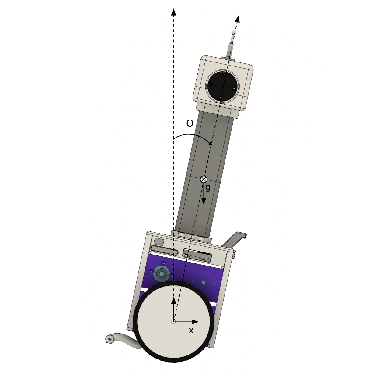
This setup is unstable, since any uncontrolled pitch will cause the robot to tip over. Our primary control goal is to minimize theta (stay upright). Additionally, we'd like to be able to command a velocity forward or backward using our FlySky RC from before. So our controller will need to carefully command pitch angle to speed up when we want to, but without tipping over.

Equations of Motion

As mentioned earlier, we'll focus on the pitch angle %%\theta %%, pitch rate %%\dot{\theta} %%, linear position %%x%% and linear velocity %%\dot{x}%% of our robot. These are two sets of coupled dynamic equations: rotational (%%\theta %%, %%\dot{\theta}%%) and translational (%%x%%, %%\dot{x}%%).

Rotational dynamics

Considering the rotational dynamics around the pivot point at the wheel axis, the moment of inertia for the system can be approximated by assuming the robot's mass is concentrated at a distance ( %%L%% ) from the pivot, leading to %%I = ML^2%% . The rotational dynamics equation, including the gravitational torque when the robot tilts by an angle ( %%\theta%% ), and assuming small angle approximations %%( \sin(\theta) \approx \theta )%% necessary to linearize the model, is derived from Newton's laws of motion:

%%ML^2\ddot{\theta} = \tau - MgL\theta %%

where:
( %%\tau%% ) is the control input torque,
( %%M%% ) is the mass of the robot,
( %%g%% ) is the acceleration due to gravity,
( %%L%% ) is the distance from the wheel axis to the robot's center of gravity (CG),
( %%\theta%% ) is the pitch angle of the robot from the vertical,
( %%\ddot{\theta}%% ) is the angular acceleration of the robot.

Solving for ( %%\ddot{\theta}%% ), the angular acceleration, we get:

%%\ddot{\theta} = \frac{\tau}{ML^2} - \frac{g\theta}{L}%%

This equation describes how changes in pitch rate ( %%\ddot{\theta}%% ) depend on the applied torque (%%\tau%%) by the motors and the current pitch angle (%%\theta%%).

Translational dynamics

The translational dynamics of the robot can be analyzed by considering the forces acting in the horizontal direction. Assuming the robot is a rigid body and no other external forces except the control force ( F ) and the gravitational force acting when the robot tilts, the translational dynamics are:

%%M\ddot{x} = F - Mg\sin(\theta)%%

Considering small angle approximations ( %%\sin(\theta) \approx \theta%% ), the equation simplifies to:

%%M\ddot{x} = F - Mg\theta%%

where:
( F ) is the control force applied to the wheels,
( M ) is the mass of the robot,
( g ) is the acceleration due to gravity,
( %%\theta%% ) is the pitch angle of the robot from the vertical,
( %%\ddot{x}%% ) is the horizontal acceleration of the robot.

Solving for ( %%\ddot{x}%% ), the horizontal acceleration, we get:

%%\ddot{x} = \frac{F}{M} - g\theta%%

This equation describes how the horizontal acceleration ( %%\ddot{x}%% ) is affected by the control force ( F ) and the gravitational component due to the robot's tilt angle ( %%\theta%% ).

State-space model representation

Now that we have our equations of motion, we can populate a state space representation of dynamics. The standard representation is:

%% \dot{\mathbf{x}} = A\mathbf{x} + B\mathbf{u}%%

Where Ax represents the natural dynamics of the system, and Bu represent the influence of control input. In this representation, x is the vector of our state variables, and u is the vector of our control inputs:

%%\mathbf{x} = \begin{bmatrix} x \\ \dot{x} \\ \theta \\ \dot{\theta} \end{bmatrix}, \quad \mathbf{u} = \begin{bmatrix} F \\ \tau \end{bmatrix}%%

The system matrix (A) describes how the state dynamics play out on their own, and the input matrix (B) describes how control inputs directly affect each state:

%%A = \begin{bmatrix} 0 & 1 & 0 & 0 \\ 0 & 0 & -g & 0 \\ 0 & 0 & 0 & 1 \\ 0 & 0 & \frac{g}{L} & 0 \end{bmatrix}, \quad B = \begin{bmatrix} 0 \\ \frac{1}{M} \\ 0 \\ -\frac{1}{ML^2} \end{bmatrix}%%

Our A matrix describes a system where position (x) depends only on the x velocity. Velocity depends on %%-g\theta%%, since a positive pitch angle tends to push the robot backwards. We also say %%\theta%% depends only on %%\dot{\theta}%%, and %%\dot{\theta}%% depends on %%\frac{g\theta}{L}%%, since a positive pitch angle creates a positive torque inducing %%\dot{\theta}%%.

LQR Controller Design

Now that we have a state space representation of our system, we can use Python's control library to design an LQR controller to stabilize our robot. In Pictorus, this is super easy. We just boot up our in-browser Python terminal and determine the control gains vector we'll use in real time. All we need to do is specify A, B, Q and R matrices, and the control.lqr function returns optimal gains K. Clicking "Save & Run" executes our Python script, and exposes any variables returned by our script to our model:

Remember that all of our apps in Pictorus compile to memory-safe Rust, so we use Python as a scripting and analysis tool to generate matrices we'll need in the compiled app. In the app, all we do is create an error vector from our measured states and take the dot product with our LQR gains (C) computed by Python:

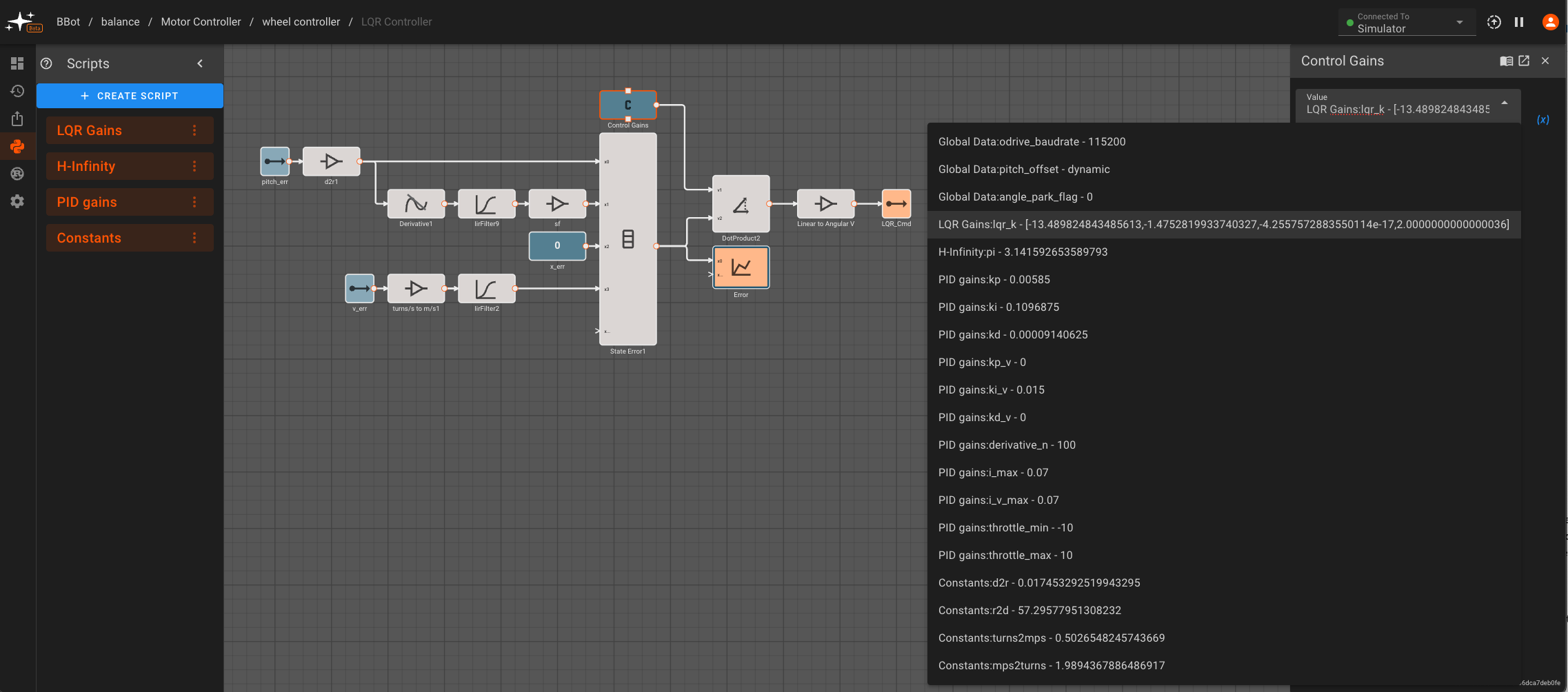
We feed in the same velocity and tilt angle errors we used for PID in our previous blog post, taking a derivative for %%\dot{\theta}%% and converting to the correct units used in our model (meters/s, radians). We also do some light filtering to the inputs in order to smooth out noise or any step changes.

Let's review the Python script shown in the animation above:

import numpy as np
import control

# System Parameters
g = 9.81  # acceleration due to gravity (m/s^2)
l = 0.126   # length to the center of mass (m)
m = 5.3   # total mass (kg)
r = 0.08  # Wheel radius (m)
max_velocity = 1.0  # Maximum velocity corresponding to full stick input
THROTTLE_GAIN = 1.0  # Mapping LQR control output to Throttle input

A = np.array([[0, 1, 0, 0],
              [g/l, 0, 0, 0],
              [0, 0, 0, 1],
              [-g/m, 0, 0, 0]])
print(A)

B = np.array([[0],
              [- 1 / (m * (l ** 2))],
              [0],
              [ 1 / m]])

# Weighting matrices
Q = np.diag([0.8, 0, 0, 2])  # Penalizing theta, theta_dot, x, and x_dot
R = np.array([[0.5]]) # Penalizing control effort

# Calculate the LQR gain matrix K
# This is what our Python script returns.
K, _, _ = control.lqr(A, B, Q, R)

return {'lqr_k': K[0]}

We described the derivation of matrices A & B earlier in this post. You'll notice we re-arranged the variable order, but the equations are the same.

The Q matrix is where we specify weights for each state variable. You can see we're only penalizing theta and velocity (x_dot). Since they use different units it's a little challenging to grasp, but a single degree of pitch error is penalized about the same as 5 cm/s velocity error.

The R matrix is where we apply arbitrary penalty to control. This is art as much as science, and we found we could dial down R to 0.50 and still get reasonable control for significantly less effort than R of unity. This should help prevent draining batteries and wearing out motors unnecessarily.

Hardware-in-the-Loop Tuning

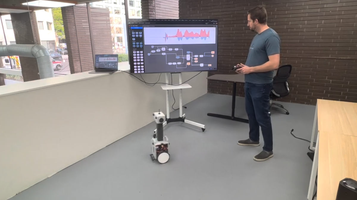
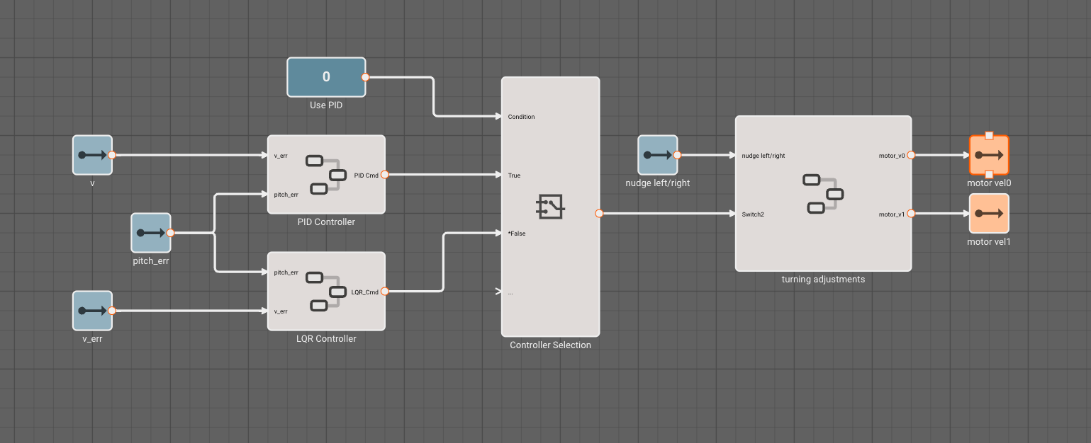
Now that we've implemented our LQR controller, we make PID vs LQR a toggle within our app. This is pretty cool, because it allows us to switch between the two and evaluate performance:

Pictorus really shines when it's time to deploy software. In particular, if your laptop and vehicle are both connected to the same WiFi network, telemetry can stream directly between them, and a higher resolution stream with about 1s latency kicks in:

Conclusions & Next Steps

It was really easy to upgrade our simple PID controller to a more sophisticated LQR controller using Python in browser. Real-time hardware in the loop testing let us dial in the control penalty (R) and weights (Q) to get a smooth, low-power controller in a matter of minutes.

From here, we could potentially explore some more advanced, robust control patterns (such as H-Infinity) using the same Python controls library. But robust control might be overkill for this robot as it stands today.

A lot of our development effort right now is going towards our distributed embedded workflow, so this robot is currently getting redesigned to carry multiple embedded processors, so we can show off programming an entire system of devices from the cloud. Stay tuned!