Designing a Self-Balancing Robot with Pictorus
In this post we’ll cover the design of a two-wheeled self-balancing robot - a classic control systems design challenge. We’ll assemble the robot hardware from accessible off-the-shelf electronics and 3D printed parts and design a controller in a Pictorus app.
Design Overview
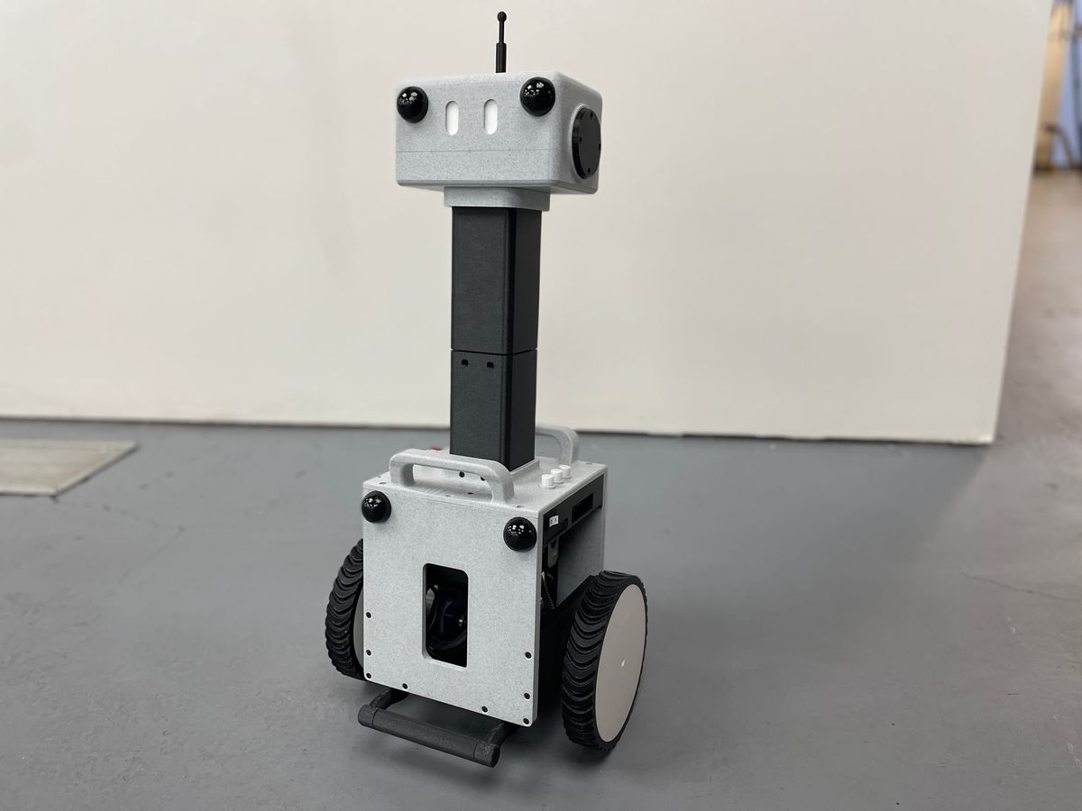
The goal of a two-wheeled self-balancing robot is simply to keep itself upright. Typically, a balancing robot has an onboard sensor to detect its current tilt angle, and motor controllers that adjust wheel velocity to correct a given tilt. Without any control input, the robot will simply fall over.
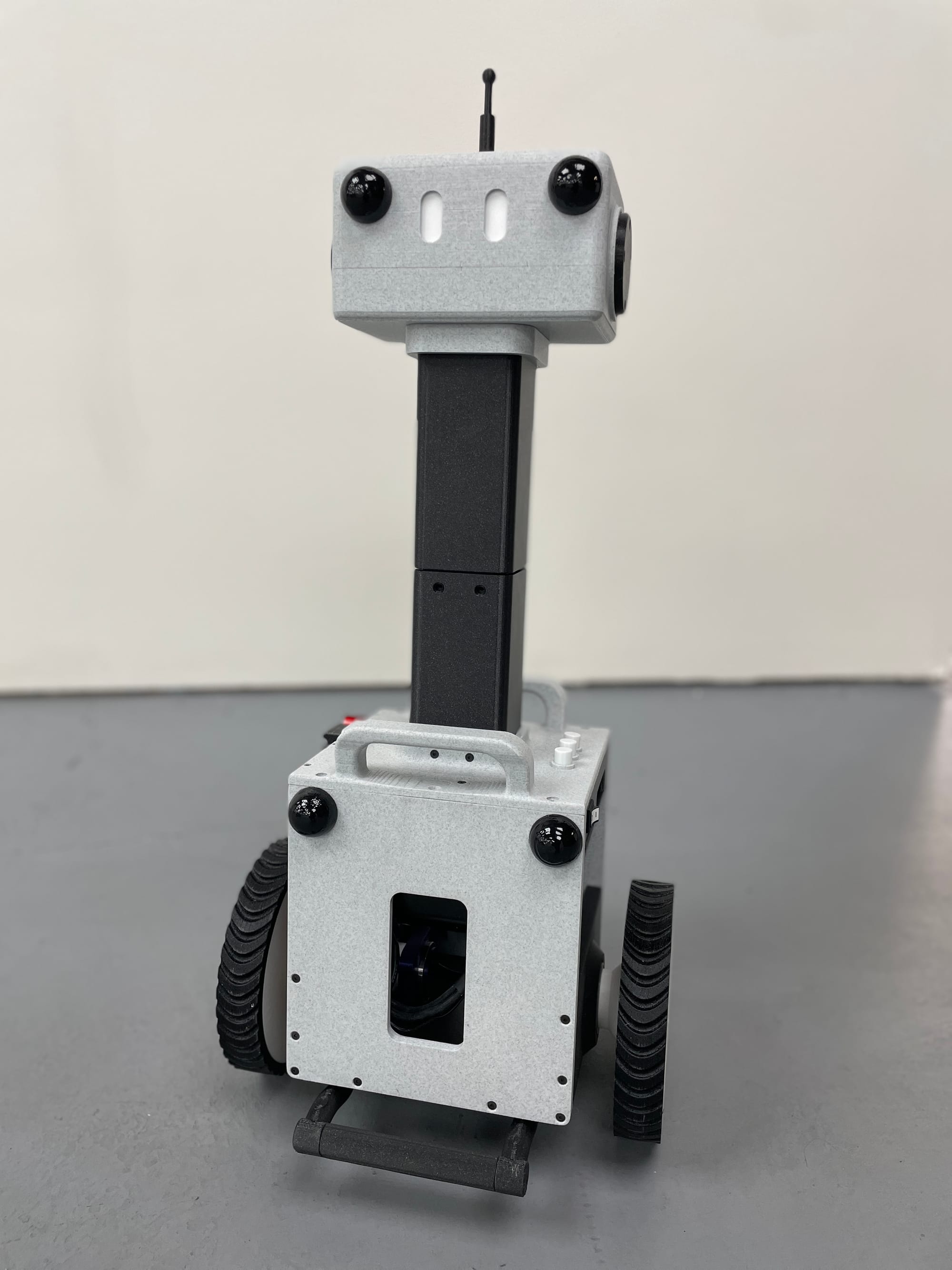
Balancer robot starting up
This system is modeled as an inverted pendulum in typical controls theory literature - having a center of mass above its wheels’ axis of rotation. Given its inherently unstable nature, the system is a great test case for different controller designs (PID and LQR to name a couple) as well as control systems modeling tools.
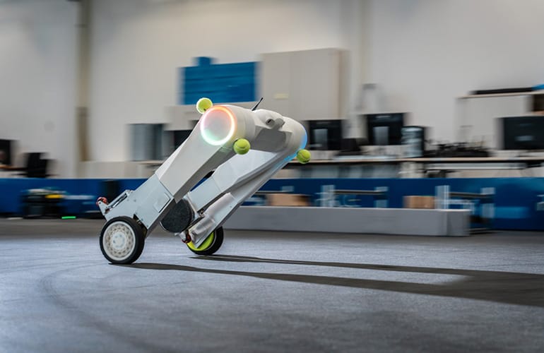
In addition to encountering self-balancing systems in controls theory literature, we often see real-world examples of this design in telepresence robots, segways, and even in some sleek transporter robots such as the evoBOT.
Robot Design
Our system’s main components consist of high-speed brushless DC motors to react to disturbances (balanced with enough torque to handle the robot’s mass), motor controllers, a sensor to measure tip/tilt and an RC transmitter and receiver to steer the robot. On the computing side, we will first read our robot's current tip/tilt values and a user's remote control commands using an onboard computer or microcontroller. We should then calculate an appropriate motor velocity for staying upright and steering according to our input, and finally we will send these velocity commands to our motors via controller boards.
Here is a list of the main components we will use to achieve this:
- Raspberry Pi4
- Adafruit 9-DOF Orientation IMU Fusion Breakout - BNO085
- ODrive S1 motor controller (x2)
- ODrive 8192CPR encoder (x2)
- ODrive D6734 150kV motor (x2)
- T5 timing belt (x2)
- T5 pulley (x2)
- 22.2 V Li-Po battery (for motors)
- PiSugar S Plus portable UPS (for RPi)
- FPVDrone Mini Receiver
Our robot’s relative scale and core mechanical components are inspired by YouTuber James Bruton’s balancing robot. We dressed the design up a bit to add our own style as well as implemented our own set of control electronics and software. We also added parking rests to hold our robot when powered off. It's main assembly consists of 3D printed parts as well as relatively low cost motors and their controllers from ODrive - making this an accessible build for a rapid prototyping lab.
A few design features that help the controllability of this robot are:
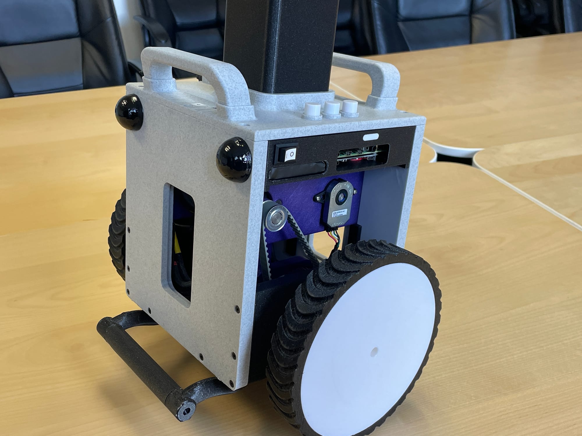
- High(enough) center of mass - achieved by moving heavy motors above the wheels and using a pulley system to turn the wheels. A LiPo battery is also placed just above the motors to keep the CoM ~0.5ft above the wheels’ axis of rotation. This makes the system respond more slowly to any torque it experiences - such as the force of gravity tipping it over. This also means we also need more torque by the motors to recover from tipping, but we can size the motors appropriately.
- Large wheels with treads. This increases surface contact and the robot’s ability to cover ground - and catch itself - more quickly.
- Fast (though definitely a bit overpowered) BLDC motors. The upside is that we can size our robot up in a future revision!
Robot Assembly and Component Testing
As previously mentioned, all of our parts were 3D printed in house, including tires out of flexible filament! We start by putting together our wheel assembly and baseplate, then slotting in our motor assembly and ensuring that the T5 timing belts are tensioned enough against the wheel and motor pulleys.
Securing motors to brackets
Assembling left wheel components
Tensioning left wheel timing belt against two pulleys
After configuring the ODrive controllers for our system, we can test out the basic inputs and outputs on a breadboard - confirming that we can talk to the motor controllers and change the speed of motors based on a measured IMU value. Eventually we’ll tune a controller to compute a wheel speed based on tilt, but for now this is sufficient to test all the basic connections.
Testing ODrive BLDC motor response to tilt in a Pictorus app
Once we’ve verified that all of the connections work on a breadboard, we solder up a pi protoboard with our components. All of the electronics fit snugly within the robot’s main body, with a battery sitting in the post just above this main enclosure.
Finally, we add some auxiliary components to the main body including two parking rests to allow our robot to plop over safely if it’s turned off, some indicator LEDs, and a couple carrying handles.
The final section is the robot’s “head” which, for now, is a visual placeholder that adds a bit of character to our balancing bot. Eventually, we can use this section for camera vision or other sensor add-ons.
Balancing App Design
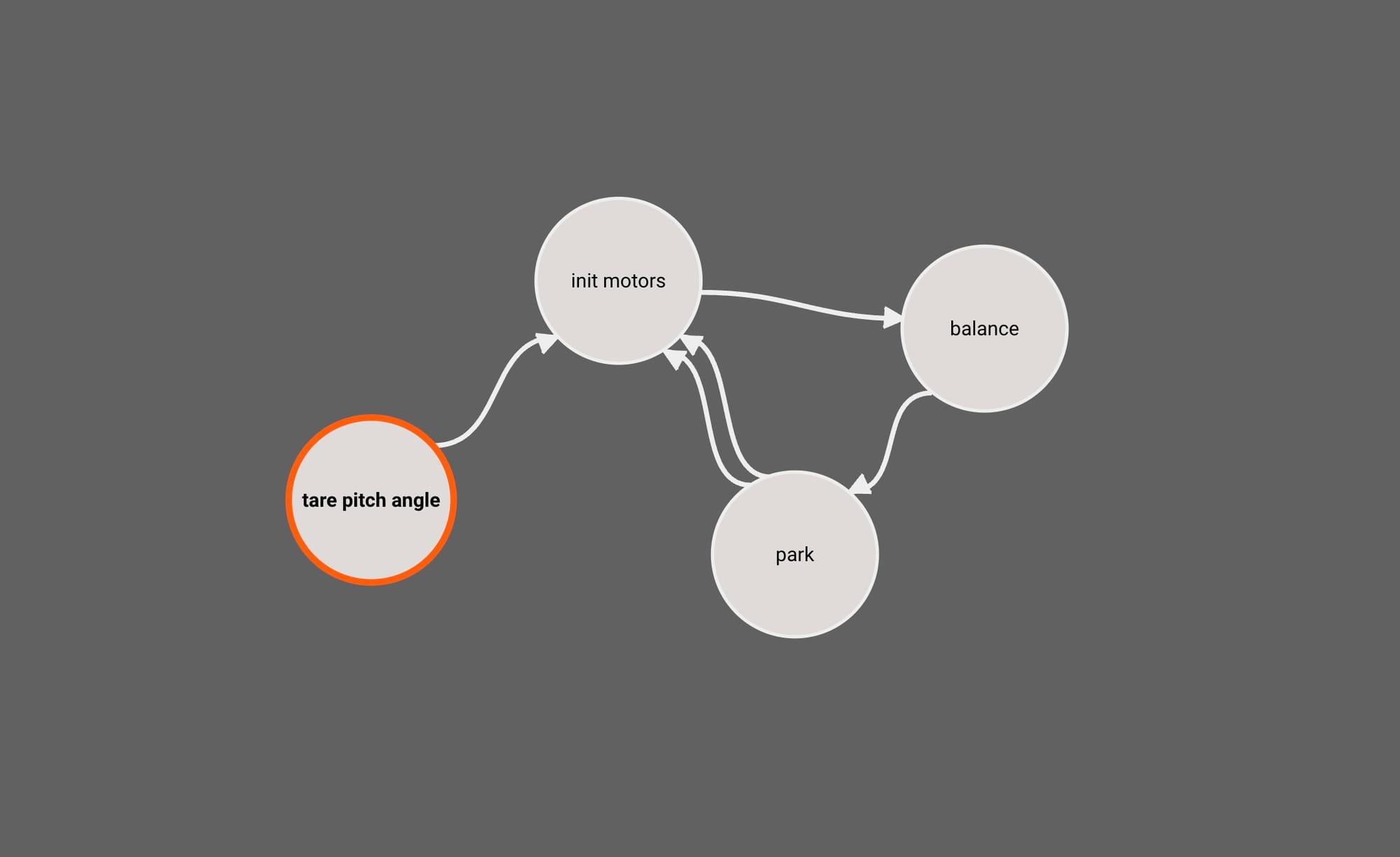
Our app will consist of four different states:
- Tare Pitch Angle
- Initialize Motors
- Balance
- Park
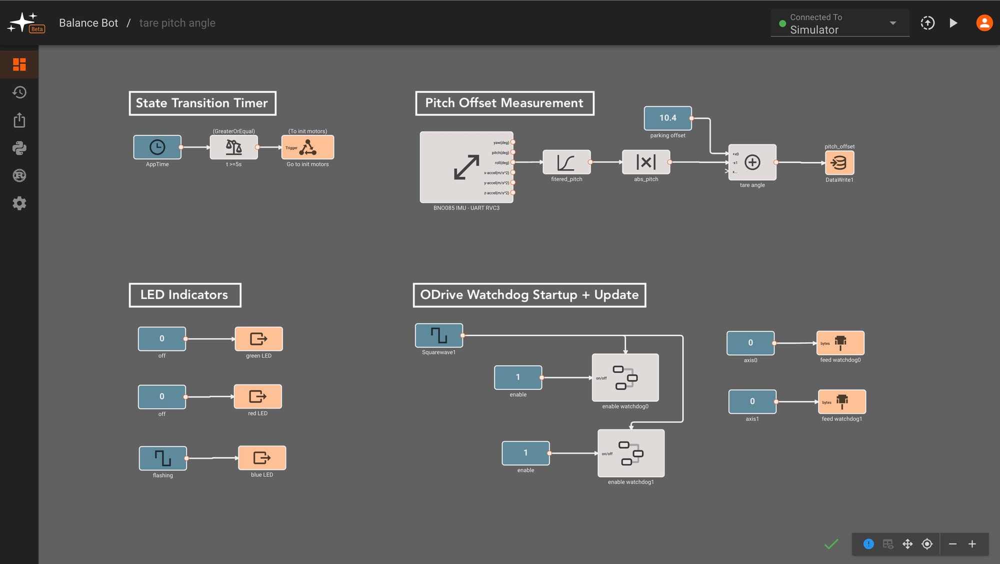
The first two states are pretty straightforward. In the Tare Pitch Angle State, we’ll measure any bias in the IMU measurement against a known reference angle. We’ll do this by reading the average IMU value over a few milliseconds as the robot leans on its parking rest. We subtract the measured value from a known parking angle to get a bias in measured pitch angle to reference later.
The Initialize Motors State simply initializes the ODrive motor controllers to switch out of idle to closed loop control - allowing us to send velocity commands to the motors in the next state. We split this out in order to re-enable motors after entering the park state, skipping the pitch taring step.
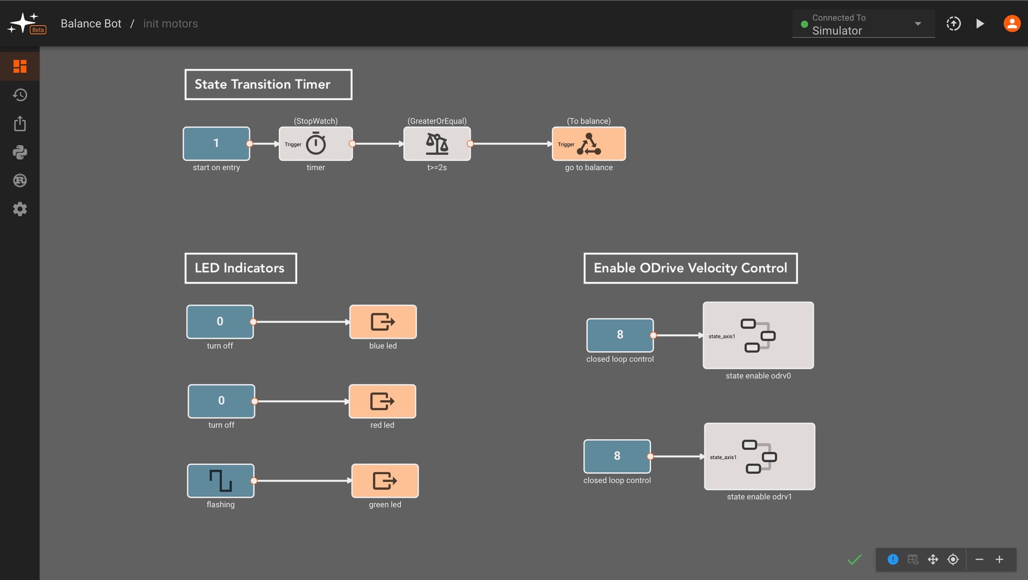
We also attach indicator light patterns to each of these states - flashing blue for IMU zeroing and flashing green for ODrive startup. This is helpful to discern which state of the app we're in.
LED indicators for boot-up (blue/flashing green), balancing (solid green), and park (red)
As we move into the Balance State, the indicator light turns to solid green and we start running the balancing control code. We’ll take a closer look at this state in the next section.
The final state is the Park State, which we enter if Switch A on our controller is flipped or we detect a pitch angle that indicates we have tipped over. If Switch A switched is flipped back up, our app interprets this as a "try again" command, moving back to the balancing state.
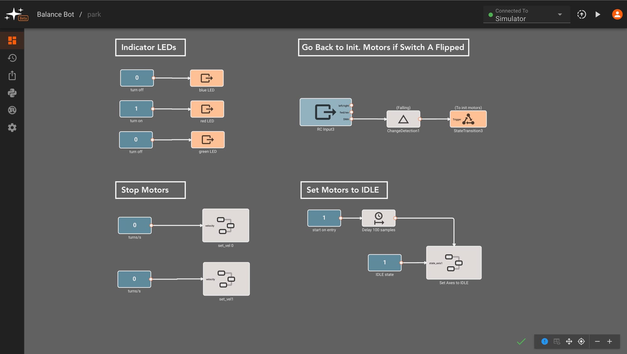
Switch control for park<>balance transition
Controller Design
We’ll be using closed loop control for our balancing robot, enabling our robot to adjust its motor speeds and achieve an upright state on its own. We could in theory control output torque or position, but we found velocity control to work well for our design. We’ll experiment with two types of controllers - PID (Proportional, Integral, Derivative) and LQR (Linear Quadratic Regulation). We’ll go over the PID controller design in this blog post, and cover LQR in the next post.
Our controller inputs and outputs are fairly straightforward - we measure tilt from an Adafruit BNO085 breakout board, interpret desired setpoints from a FlySky remote control receiver, and output velocity commands to the two ODrive motor controllers via serial communication.
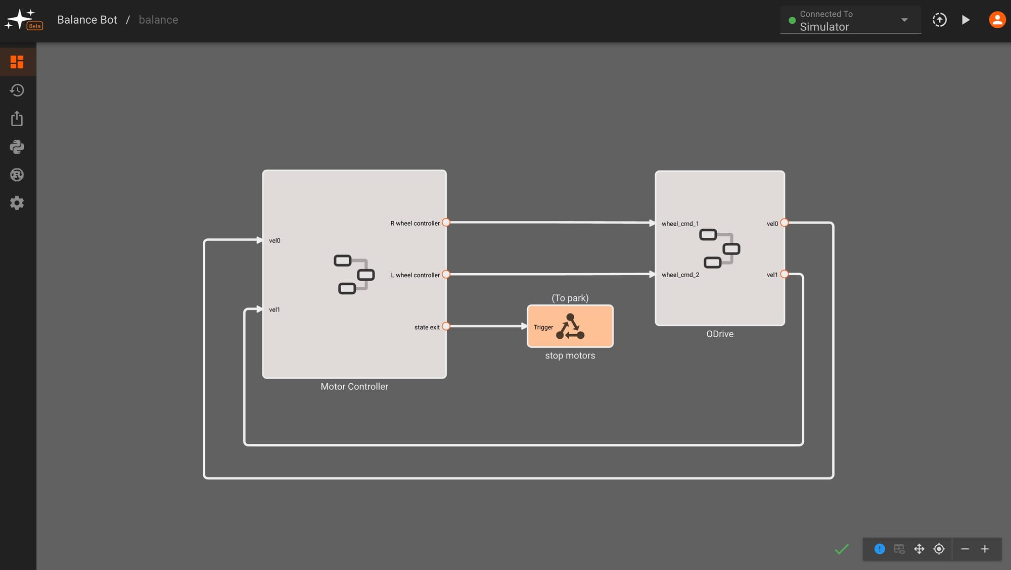
High-level controller view
Here's the top-level view of our balance state, showing velocity control outputs being sent to the ODrive motor controllers and measured wheel velocity feedback. We can also see a state transition or "abort" command that stops the motors and parks the robot.
Let's take a look at the motor controller component diagram. On the left side we take in RC input commands for steering, computing desired wheel velocities and a pitch angle based on this input, then feeding these into a controller block that makes adjustments to achieve the target motions. We also see more details for our state exit conditions, showing that we transition to the park state if we tip past a certain pitch angle threshold or our user flips a state exit switch on our remote control.
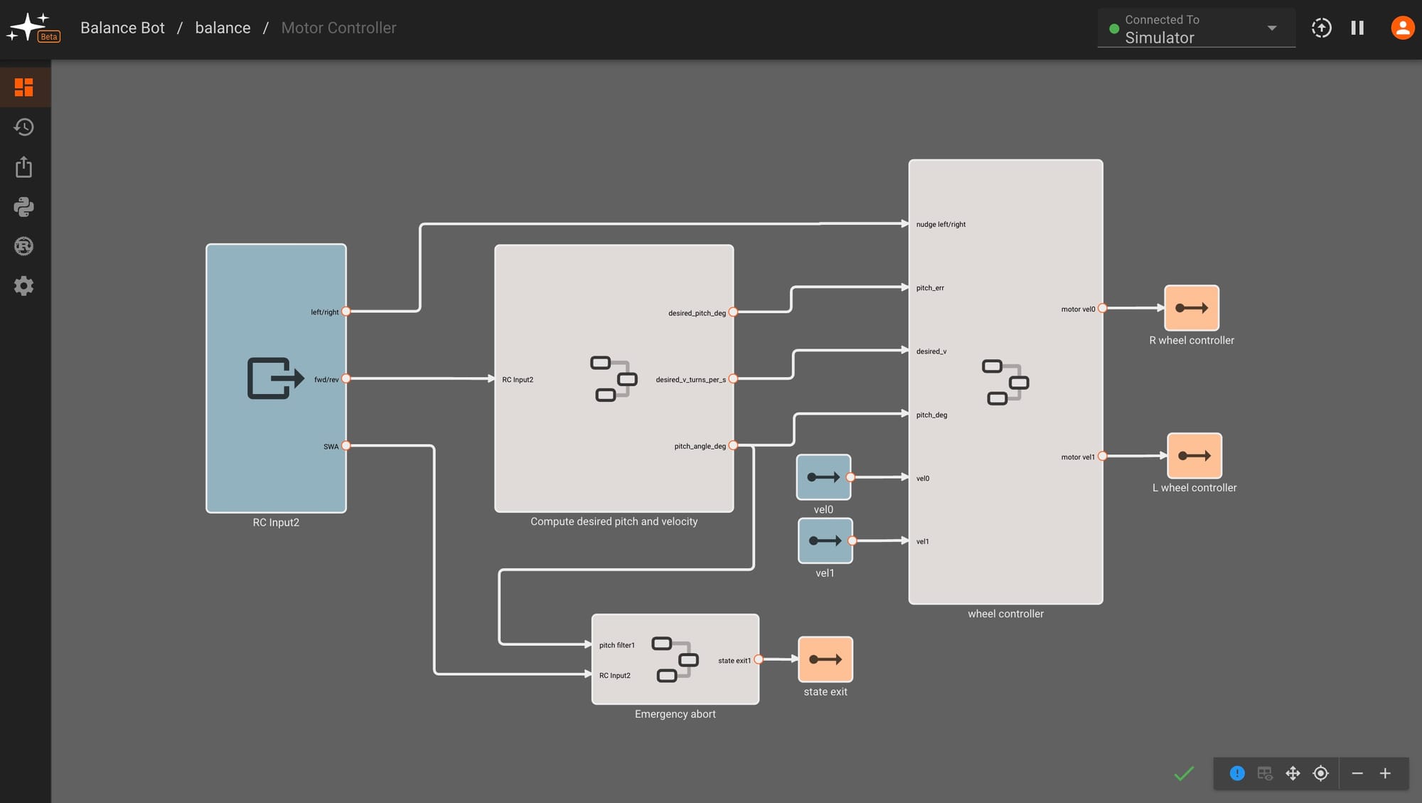
In the next section, we'll dig deeper into the setpoint (labeled "compute desired pitch and velocity") and "wheel controller" sections of this state.
Mapping RC Input to Desired Setpoint + Computing Pitch, Velocity Error
The first step in our balancing system is to map an RC input to a desired setpoint for our controller and compute our current offset from this target. This setpoint will affect both our target pitch angle and target velocity. The simplest case is where we want the robot to remain perfectly upright and stay in place. For this, we compute the difference (error) between a measured tilt angle from our IMU and a desired zero tilt angle. The controller will then output motor velocities to minimize the error we just calculated and nudge our tilt angle back to zero - keeping our robot in place and upright.
In order to move our robot, we introduce an offset in our target tilt angle. If we want our robot to move forward - a positive angle offset, our controller output, and gravity work together to push our robot forward. We also add in a separate controller that corrects for velocity error, rather than tilt angle error, to help nudge our velocity towards the user's desired input speed and correct remaining errors from our angle controller. We'll dive deeper into controller specifics in the following section.
To turn, we introduce a difference in speed between the two wheels, also known as differential drive. The left/right stick inputs are fed into the wheel controller and added in as offsets after all of our balancing control computations. The exact gains mapping all of our RC values to wheel speeds were tuned empirically.
The following video gives a high-level rundown of input mapping and error calculation in our app. Note that velocity error is computed within the "wheel controller" component:
Computing angle, velocity setpoints and errors
These errors are then fed into our wheel controller component, which has the ability to switch between PID and LQR control. In this video we also see wheel speed adjustments for turning at the end, just before the component outputs:
Controller inputs and outputs, highlighting choice of PID controller
In the next section, we'll take a closer look at the PID controller design and tuning.
PID Control Overview
We started off with PID control implementation - given its universality in stabilization designs, approachability, and ease of implementation in Pictorus (there’s a block for it!). We'll introduce two PID controllers - one for angle control and one for velocity control - that will work in tandem to balance and steer our robot.
Generally speaking, a PID controller reads an error input (tilt degrees or velocity) and computes a desired actuator output response (motor motion) based on the input value - attempting to bring this error to zero. The output response is based on the controller’s tunable proportional, integral, and derivative components.
Mathematically, the controller can be described as:
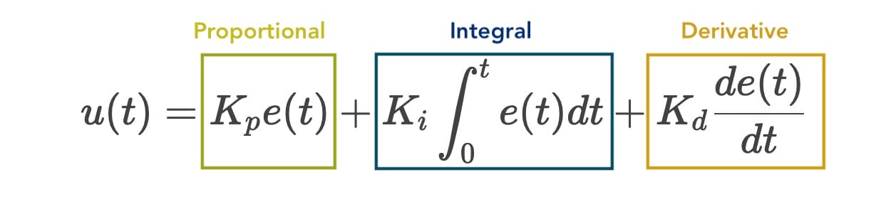
For the purposes of our balancing app, we need to understand the effect that each component has on the output. Let's consider the simplest case of making our robot stay upright (zero tilt) without moving, and look at the effects of each component:
P: The proportional component is simply a multiplier that acts on our error (tilt angle), providing faster wheel speeds for higher tilt angles and minor adjustments around zero tilt. This allows our robot to snap itself up from a parked state with a quick wheel turn and then settle around an upright position with small wheel movements.
I: The integral component sums up any tilt angle error over time, slowly accelerating the wheels until we reach a target tilt of zero - this component should also account for any remaining offset that’s not fixed in the proportional response.
D: Finally, the derivative component considers the rate of change of the tilt angle error, trying to damp out any remaining oscillations and prevent the robot from overshooting its target upright position.
To effectively balance our robot, we need to tune the constants associated with each component of our PID controllers - %%K_{p}, K_{i},%% and %%K_{d}%%.
In Pictorus, we can find each of these terms by clicking on the PID block and viewing its parameters. We also have the option to adjust the number of samples we are using to compute the derivative component as well as a limit for the integral component to prevent integral windup.
PID Block parameters
We started off with an angle-only PID controller but found that our robot could still inch forward in an upright position even when we returned our RC stick position back to zero. To prevent this, we introduced a second PID controller for velocity. For this velocity-only controller, we zeroed out our Proportional and Derivative terms, making this a slowly correcting Integral controller to settle our velocity at zero or a target velocity from our RC transmitter. Careful tuning is required to weight angle correction more heavily here - ensuring that overall control is more aggressive to correct angle disturbances (keeping our robot upright) rather than velocity offsets.
Finally, we sum our two PID controller outputs, scale them to an appropriate motor velocity range, and feed them into a ‘send velocity’ component that communicates with the ODrive controller boards.
Angle-feedback and velocity-feedback based PID controllers
The result of our PID control is fairly decent, but we found that our system still showed a bit of instability particularly at faster speeds. We turned to LQR as more sophisticated method of control, given that we could model our system and work to achieve multiple goals (appropriate wheel speed and minimal tilt angle) all within one controller.
PID controlled robot